
Working with data often requires flexibility across various software platforms. Whether you’re a researcher, data analyst, or student, there are moments when you need to export from Stata to Excel.
This guide is divided into three sections. To jump directly to any of these sections, click on the link.
(1) Exporting results with the Stata’s build-in commands
(2) Creating publication quality tables using asdocx
(3) Exporting Stata data to Excel.
1. Exporting Results with Stata’s Built-in Commands
- Why and when to use Stata’s native commands.
- A detailed guide on executing these commands effectively.
- putexcel — Export results to an Excel file
- collect export — Export table from a collection
- putexcel advanced . Export results to an Excel file using adv. syntax
- xl() — Excel file I/O class
- Potential pitfalls to watch out for and how to troubleshoot them.
1.1 Why built-in commands to export from Stata to Excel
Stata’s native commands offer a direct method to export from Stata to Excel. Since Stata Corp. is responsible for maintaining and updating these commands, users can be confident that these commands are available to everyone. This ensures that sharing the code with colleagues or other researchers is straightforward. However, the downside is that these commands are often designed to cater to a broad research community, making them somewhat generic. Customizing them requires additional coding efforts.
1.2 Stata built-in commands to export results to Excel
The Stata built-in commands can be categorized into four categories. These are: (1) putexcel (2) collect export (3) putexcel advanced (4) xl() class. These are discussed below in detail.
putexcel command
putexcel is a powerful command in Stata that allows users to write Stata expressions, matrices, tables, images, and returned results directly to an Excel file. Additionally, putexcel can format the cells in the worksheet. This functionality is especially useful for automating the exporting and formatting of Stata estimation results. It supports both the older Excel 1997/2003 (.xls) files and the newer Excel 2007/2010 and beyond (.xlsx) files.
Syntax Details:
Before writing results to an Excel file, putexcel requires that you declare the Excel file as the destination for subsequent putexcel commands. The syntax is:
[code]putexcel set filename [, set_options] [/code]
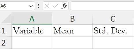
Now we can write text, returned results, matrices, or images to the Excel file. For example, to write the text “Variable”, “Mean”, and “Std. Dev.” to cells A1, B1, and C1 :
Write text to Excel
[code]* Set file ‘Table 1.xlsx’
. putexcel set “Table 1.xlsx”
* Write text
. putexcel A1 = “Variable”
. putexcel B1 = “Mean”
. putexcel C1 = “Std. Dev.”[/code]
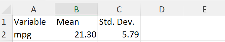
Write returned results to Excel
[code]. sysuse auto, clear
. summarize mpg
. return list
. putexcel A2 = “mpg”
. putexcel B2 = `r(mean)’, nformat(number_d2)
. putexcel C2 = `r(sd)’, nformat(number_d2)[/code]
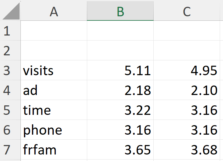
Write matrix to Excel
You can use putexcel in Stata to create tables in Excel by using the matrix() output type. The following example is from Stata Manual. Suppose we want to create a table of means for each variable for each value of female. We can use tabstat with the save option, that will write the tabstat results to r(Stat1) , r(Stata2), and r(StatTotal) matrices.
[code]. use https://www.stata-press.com/data/r18/website
. tabstat visits ad time phone frfam, by(female) save[/code]
We convert the row vectors r(Stat1) and r(Stat2) that have the means so that the values are placed in columns beneath each title. For males, our first matrix to export, we opt for the rownames option to have the variable names displayed. We target A3 because we desire the values in B3 and the matrix’s row names in A3. We employ nformat(number d2) to present the means with two decimal points. For females, there’s no need to mention the names again; we merely pinpoint the desired cell for the data placement.
[code]. qui tabstat visits ad time phone frfam, by(female) save
. matrix male = r(Stat1)’
. matrix female = r(Stat2)’
. putexcel A3 = matrix(male), rownames nformat(number_d2)
. putexcel C3 = matrix(female), nformat(number_d2)[/code]
 asdocx: Create Publication-Quality with ease
If your goal extends beyond basic exporting and you want to save time by avoiding the complex coding of syntax structures like putexcel or layouts, asdocx is the best available option. In this section, we will explore:
- An introduction to the
asdocxcommand and its relevance. - A tutorial on generating top-notch tables tailored for professional use.
- Tips and tricks to enhance the visual appeal and accuracy of your tables.
Introduction to asdocx
asdocx is a premium version of asdoc. It is currently avaiable for $9.99, with plenty powerful features. Using asdocx is pretty easy. You need to add just asdocx as a prefix to Stata commands. For example, we use the sum command to find summary statistics of all numeric variables in the dataset. We shall add just asdocx as a prefix to sum .
In the following paragraph, I show the use of asdocx with some of key Stata commands.
Export summary statistics to excel
asdocx creates comprehensive tables of summary statistics. asdocx provides four distinct methods for generating tables of these statistics. These methods are detailed below, accompanied by examples and relevant options.
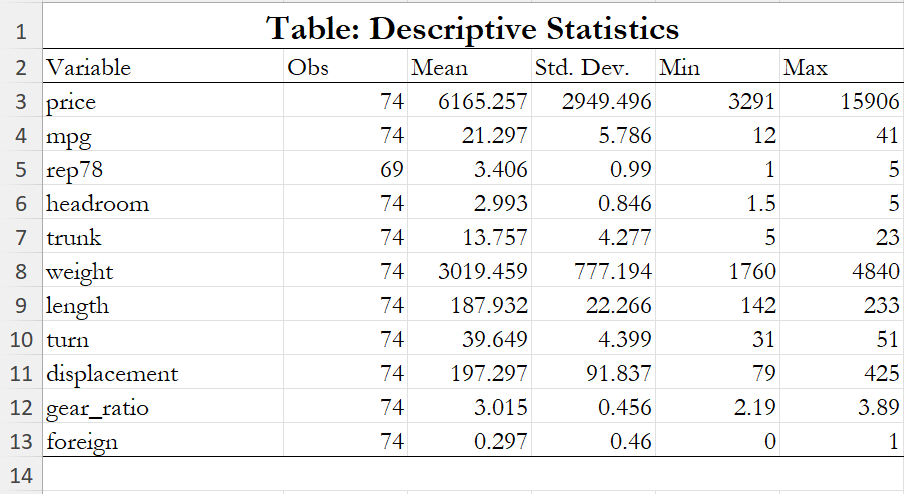
1. Default tables of summary statistics
By default, asdocx uses the summary statistics reported by Stata’s summarize command. So, without specifying any options, asdocx will generate a table with statistics including N, mean, standard deviation, min, and max.
[code]sysuse auto, clear
asdocx sum, replace save(Descriptive Statistics.xlsx)[/code]
[code]* Summary / descriptive: reporting variable labels
asdocx sum price mpg rep78 headroom trunk, save(Table.xlsx) label replace
* Summary / descriptive statistics with [if] [in] conditions
asdocx sum price mpg rep78 headroom trunk if price>4000
* Control decimal points with the dec() option
asdocx sum, dec(2)
[/code]
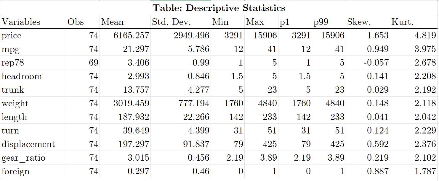
2. Detailed summary statistics
For detailed summary statistics in Stata, we typically use the summarize, detail or sum, detail commands. To create a table of these detailed statistics using asdocx, simply append detail after the comma in the asdocx sum command. By doing so, the table will include the following statistics: observations, mean, standard deviation, minimum, maximum, 1st percentile, 99th percentile, skewness, and kurtosis.[code]* Create detailed summary statistics
asdocx sum, detail save(Myfile.xlsx) replace[/code]
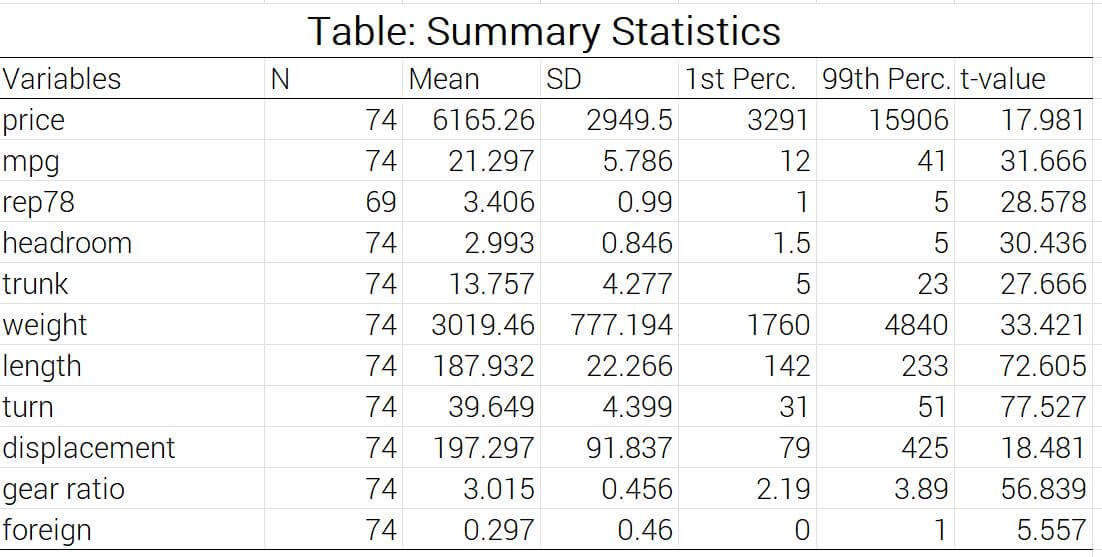
3. Custom summary statistics
To make a table of a specific combination of statistics, we shall use the option statistics() with asdocx sum command. [code]
N Number of observations
mean Arithmetic mean
sd Standard deviation
semean Stanard error of the mean
sum Sum / total
range Range
min The smallest value
max The largest value
count Counts the number of non-missing observations
var Variance
cv Coefficient of variation
skewness Skewness
kurtosis Kurtosis
iqr Interquartile range
p1 1st percentile
p5 5th percentile
p10 10th percentile
p25 25th percentile
p50 Median or the 50 percentile
p75 75th percentile
p99 99th percentile
tstat t-statistics that the given variable == 0
* In the stat() option, you can write any of the above statistics
asdocx sum, stat(N mean sd tstat p1 p99)[/code]
4. Summary statistics over a grouping variable
To find summary statistics separately for each category of a grouping variable, we can use by(varname) or the prefix bysort varname: with asdocx.[code]sysuse auto, clear
asdocx sum, stat(N mean sd tstat p1 p99) by(foreign)[/code]
To enhance the page loading speed, the table created by asdocx will be displayed in HTML format below. Given that asdocx has the capability to export to various formats such as Word, Excel, LaTeX, and HTML, the subsequent table is a direct replication from asdocx, presented without any alterations.
| N | Mean | SD | 1st Perc. | 99th Perc. | t-values | |
|---|---|---|---|---|---|---|
| Car origin: Domestic | ||||||
| price | 52 | 6072.423 | 3097.104 | 3291 | 15906 | 13.425 |
| mpg | 52 | 19.827 | 4.743 | 12 | 34 | 28.483 |
| rep78 | 48 | 3.021 | 0.838 | 1 | 5 | 24.985 |
| headroom | 52 | 3.154 | 0.916 | 1.5 | 5 | 23.994 |
| trunk | 52 | 14.75 | 4.306 | 7 | 23 | 24.406 |
| weight | 52 | 3317.115 | 695.364 | 1800 | 4840 | 33.919 |
| length | 52 | 196.135 | 20.046 | 147 | 233 | 68.581 |
| turn | 52 | 41.442 | 3.968 | 31 | 51 | 75.723 |
| displacement | 52 | 233.712 | 85.263 | 86 | 425 | 19.325 |
| gear ratio | 52 | 2.807 | 0.336 | 2.190 | 3.580 | 58.862 |
| foreign | 52 | 0 | 0 | 0 | 0 | |
| Car origin: Foreign | ||||||
| price | 22 | 6384.682 | 2621.915 | 3748 | 12990 | 12.525 |
| mpg | 22 | 24.773 | 6.611 | 14 | 41 | 18.364 |
| rep78 | 21 | 4.286 | 0.717 | 3 | 5 | 27.386 |
| headroom | 22 | 2.614 | 0.486 | 1.5 | 3.5 | 25.891 |
| trunk | 22 | 11.409 | 3.217 | 5 | 16 | 15.950 |
| weight | 22 | 2315.909 | 433.003 | 1760 | 3420 | 28.439 |
| length | 22 | 168.545 | 13.683 | 142 | 193 | 59.238 |
| turn | 22 | 35.409 | 1.501 | 32 | 38 | 113.933 |
| displacement | 22 | 111.227 | 24.881 | 79 | 163 | 22.079 |
| gear ratio | 22 | 3.507 | 0.297 | 2.980 | 3.890 | 52.855 |
| foreign | 22 | 1 | 0 | 1 | 1 | |
| Notes: | ||||||
Export table of correlations to Excel
asdocx can create tables almost for all Stata commands related to correlations such as simple correlations, pairwise and partial correlations, interclass correlation, and tetrachoric correlation. Visit the asdocx cor page to explore the myriad of features and options at your disposal for creating a correlation table. The following syntax is used for asdocx cor command:
[code]asdocx cor [varlist] [if] [in], [nonum label dec(#) asdocx_options]
*Example: correlations among all numeric variables
sysuse auto, clear
asdocx cor [/code]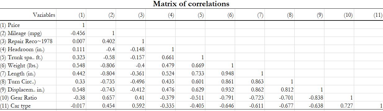
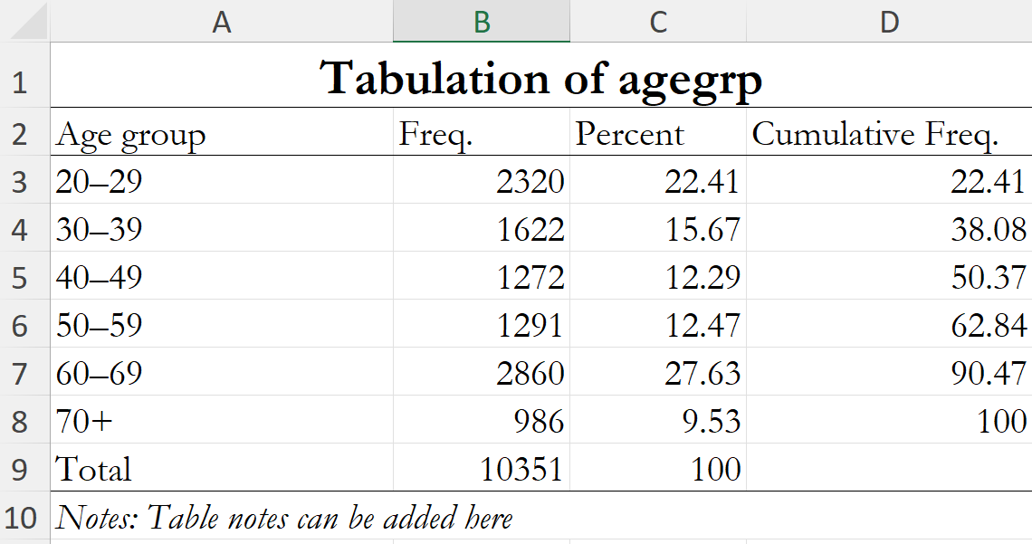
Export tabulations to Excel
[code]* use the NHS dataset from web
webuse nhanes2l, clear
* One way tabulation
asdocx tab agegrp, save(Myfile.xlsx) replace
[/code]
[code]
* Two way tabulation
* Three-way tabulation
[/code]
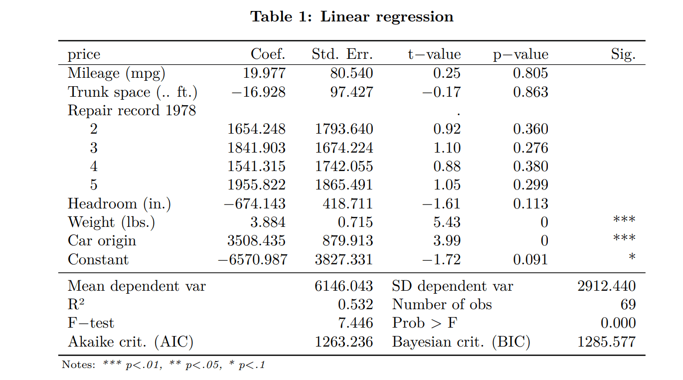
Export regressions from Stata to Excel
asdocx can create three types of regression tables. The first type is the detailed table that combines key statistics from the Stata’s regression output with some additional statistics such as mean and standard deviation of the dependent variable etc. This table is the default option in asdocx. The second table is the nested table that nests more than one regressions in one table. The third table is the wide table that reports regression components in a wide or row format. You can explore these on thier respective page where options and examples are discussed in detail.
[code]* Detailed regressions
sysuse auto, clear
asdocx reg price mpg trunk i.rep78 headroom weight foreign, label replace
[/code]
3. Exporting Stata Data to Excel
Sometimes, the need is as simple as transferring your Stata dataset to Excel, either for sharing, further analysis, or visualization. This section will cover:
- The advantages of having your data in Excel format.
- A hands-on guide to ensure a smooth data transfer from Stata to Excel.
- export — Overview of exporting data from Stata
- Solutions to common issues faced during the export process.