Publication grade nested regressions table in Stata | asdocx
Publication grade nested regressions table in Stata | asdocx
- Default case
- Report t-statistics, standard errors, or p-values
- Report t- and p-value or ci to the right-side of coefficients
- Reporting variable Labels
- Add statistics from e()
- Add text or custom statistics
- Keep or drop variables from table
- Start a new table with option reset
- Set decimal points separately for coefficient and t-value / p-values
- Add custom text / statistics
- Use option by() for group-regressions
- Suppress se / t-value/ p-values with notse option
asdocx can create three types of regression tables. The first type is the detailed table that combines key statistics from the Stata’s regression output with some additional statistics such as mean and standard deviation of the dependent variable etc. This table is the default option in asdocx. The second table is the nested table that nests more than one regressions in one table. The third table is the wide table that reports regression components in a wide or row format. In this post, I discuss the nested tables, their options, and examples.
syntax
[bysort varname :] asdocx depvar indepvars [if] [in], [asdocx_options
                  regression_options]
Following is a list of asdocx options that are available with the nested regressions:
| Option | Purpose |
|---|---|
| nested | to invoke creation of nested tables. |
| rep(t | se | p | ci) | to report t, standard errors, p, or confidence intervals with regression coefficients. |
| sideways | to report t, p, se, or ci values to the right-side of coefficients. Default is to report these below coefficients. |
| title(table title) | to specify the regression table title. |
| cnames(col title) | to specify column titles, default is to report the dependent variable name. |
| dec(#) | to specify the decimal places for regression coefficients; default is 3 dp. |
| dect(#) | to specify the decimal points for se, t, p, or ci. |
| add() | to add text in pairs to the title row and current regression column. |
| keep(varlist) | to keep variables in the output table. |
| drop(varlist) | to drop variables from the output table. |
| stat() | to report statistics availabe in e() macros. |
| setstars | to set custom significance level for start. Default is setstars(***@.01, **@.05, *@.1). |
| nostars | to suppress significance stars. |
| level(##) | [used with rep(ci) only] to specify custom significance level of ci. |
| eform | to report exponentiated coefficients. |
| label | to report variable labels instead of names. |
| reset | to start a new nested table. |
| alignstats | to vertically align statistics; default is to align statistics with significance stars. |
| nonum | to omit model numbers that appear at the top of columns. |
1. Default case
The option nested or nest invokes the creation of nested regression tables. Without this option, the default (detailed regression) table is created by asdocx. Let us create our first nested regression table.
* Load some example data
sysuse auto, clear

* Add first regression to the nested model
asdocx reg price trunk mpg, nest replace

* Add second regression to the nested model
asdocx reg price trunk mpg weight, nest
| Variables | (1) | (2) |
|---|---|---|
| price | price | |
| trunk | 43.559 | -65.323 |
| (88.719) | (93.625) | |
| mpg | -220.165*** | -54.917 |
| (65.593) | (86.815) | |
| weight | 1.956*** | |
| (0.71) | ||
| Intercept | 10254.95*** | 2328.163 |
| (2349.084) | (3651.422) | |
| Observations | 74 | 74 |
| R2 | 0.222 | 0.298 |
| Notes: Standard errors are in parentheses. *** p<.01, ** p<.05, * p<.1 | ||
2. Report t-statistics, standard errors, p-values or CI
Option rep() is used in combination with option nest for reporting t-values, standard errors, p-values or confidence intervals with each of the regression coefficient. Use rep(t) to report t-statistics, rep(p) to report p-values, and rep(se) to report standard errors, and rep(ci) to report confidence intervals. The default option is rep(se). Please note that option rep(t), rep(p) and rep(ci) will work only when used at the start of the nested table. This is the case either:
(i) when option replace is used or
(ii) the nested table is started for the first time.
* Load some example data
sysuse auto, clear

* Report t-statistics with option rep(t)
asdocx reg price trunk mpg, nest replace rep(t)

* Add second regression to the nested model
asdocx reg price trunk mpg weight, nest rep(t)
| Variables | (1) | (2) |
|---|---|---|
| price | price | |
| trunk | 43.559 | -65.323 |
| (0.491) | (-0.698) | |
| mpg | -220.165*** | -54.917 |
| (-3.357) | (-0.633) | |
| weight | 1.956*** | |
| (2.754) | ||
| Intercept | 10254.95*** | 2328.163 |
| (4.366) | (0.638) | |
| Observations | 74 | 74 |
| R2 | 0.222 | 0.298 |
| Notes: t-values are in parentheses. *** p<.01, ** p<.05, * p<.1 | ||
3. Report ci, se, t- or p-values sideways
Option sideways is used to report t-statistics, standard errors, p-values, or confidence intervals to the right-side of the regression coefficients. The default setting is to report them below the coefficients. In the following examples, I am creating a nested table with the following specifications.
Regression table: two logit nested regressions : option nest
Coefficients: exponentiated / odd ratios : option eform
Significance statistics: confidence interval using option rep(ci)
Placement of the significance statistics : to the right-side of the coefficients: option sideways
Variable names: reporting labels instead of names : option label
Level of confidence: 99% : option level(99)
* Load example data
 webuse lbw
 asdocx logit low age lwt i.race smoke ptl, eform nest ///
        sideways rep(ci) label level(99) replace

 asdocx logit low age lwt i.race smoke ptl ht ui, eform ///
        nest sideways rep(ci) label level(99)
| (1) | (2) | |
|---|---|---|
| Variables | birthweight<2500g | birthweight<2500g |
| age of mother | 0.973 [0.886, 1.069] | 0.968 [0.883, 1.06] |
| weight at last menstrual period | 0.985 [0.968, 1.003] ** | 0.989 [0.973, 1.006] * |
| race | ||
| black | 3.535 [0.911, 13.716] ** | 3.365 [0.885, 12.792] ** |
| other | 2.368 [0.764, 7.339] ** | 2.475 [0.833, 7.353] ** |
| smoked during pregnancy | 2.518 [0.897, 7.07] ** | 2.53 [0.93, 6.887] ** |
| premature labor history (count) | 1.719 [0.705, 4.194] | 1.914 [0.807, 4.541] * |
| has history of hypertension | 6.25 [1.052, 37.116] *** | |
| presence, uterine irritability | 2.135 [0.654, 6.971] * | |
| Intercept | 1.586 [0.071, 35.306] | 1.313 [0.072, 23.898] |
| Observations | 189 | 189 |
| Pseudo R2 | 0.142 | 0.102 |
| Notes: Confidence intervals are reported in brackets at 99%. *** p<.01, ** p<.05, * p<.1 | ||
4. Report variable labels
By default, asdocx writes variable names as the row headers. Option label can be used to report variable labels instead of variable names.
* Load some example data
sysuse auto, clear

* Add first regression to the nested model
asdocx reg price trunk mpg, nest label replace

* Add second regression to the nested model
asdocx reg price trunk mpg weight, nest label
| (1) | (2) | |
|---|---|---|
| Price | Price | |
| Trunk space (cu. ft.) | 43,559 | -65,323 |
| (88,719) | (93,625) | |
| Mileage (mpg) | -220,165*** | -54,917 |
| (65,593) | (86,815) | |
| Weight (lbs.) | 1,956*** | |
| (0,71) | ||
| Intercept | 10 254,95*** | 2 328,163 |
| (2 349,084) | (3 651,422) | |
| Observations | 74 | 74 |
| R2 | 0,222 | 0,298 |
| Notes: Standard errors are in parentheses. *** p<.01, ** p<.05, * p<.1 | ||
5. Add statistics from e()
Option stat() can be used to report additional regression statistics that are stored in macro e(). The e() macros are available after running a regression model. Since asdocx runs regression models below the surface, these macros are obtained by asdocx and can be reported by providing the macro names in option stat() without the e() part. For example, stat(rmse rss) will report the RMSE and RSS of the model. Please note that these statistics will be reported only if they are available in the e() macro. If they are not available, asdocx will highlight it as an error and report the given statistic as missing. All e() macros can be listed by typing ereturn list in Stata command window after a regression model. See the following example where I report the RMSE and adjusted r-squared, which are available in the e(rmse) and e(r2_a) macros, respectively.
* Add first regression to the nested model
asdocx reg price trunk mpg, nest stat(rmse r2_a) replace

* Add second regression to the nested model
asdocx reg price trunk mpg weight, nest stat(rmse r2_a)
| Variables | (1) | (2) |
|---|---|---|
| price | price | |
| trunk | 43.559 | -65.323 |
| (88.719) | (93.625) | |
| mpg | -220.165*** | -54.917 |
| (65.593) | (86.815) | |
| weight | 1.956*** | |
| (0.71) | ||
| Intercept | 10254.95*** | 2328.163 |
| (2349.084) | (3651.422) | |
| Observations | 74 | 74 |
| R2 | 0.222 | 0.298 |
| RMSE | 2637.591 | 2523.164 |
| Adj R2 | 0.2 | 0.268 |
| Notes: Standard errors are in parentheses. *** p<.01, ** p<.05, * p<.1 | ||
6. Drop or keep variables
keep(varlist) and drop(varlist) are alternatives; they specify coefficients to be included or omitted from the table. The default is to display all coefficients. In the following example, I shall exclude all year and industry dummies from the regression table; however, these dummies will still be included in the regression models. Please note that the prefix i. is used for factor variables. If a variable is not a factor variable, it will be written without the i. prefix.
* Load Data
use http://fintechprofessor.com/regdata.dta, clear

* Add first regression
asdocx reg y x1 x2 x3 i.year i.location, nest drop(i.year i.location) replace

* Add another regression
asdocx reg y x1 x2 x4 i.year i.location, nest drop(i.year i.location)
| Variables | (1) | (2) |
|---|---|---|
| y | y | |
| x1 | 1.315*** | 1.279*** |
| (0.25) | (0.25) | |
| x2 | 0.939*** | 1.167*** |
| (0.232) | (0.237) | |
| x3 | 1.068*** | |
| (0.227) | ||
| x4 | 1.107*** | |
| (0.232) | ||
| Intercept | 0.694*** | 0.626** |
| (0.24) | (0.244) | |
| Observations | 50 | 50 |
| R2 | 0.666 | 0.669 |
| Notes: Standard errors are in parentheses. *** p<.01, ** p<.05, * p<.1 | ||
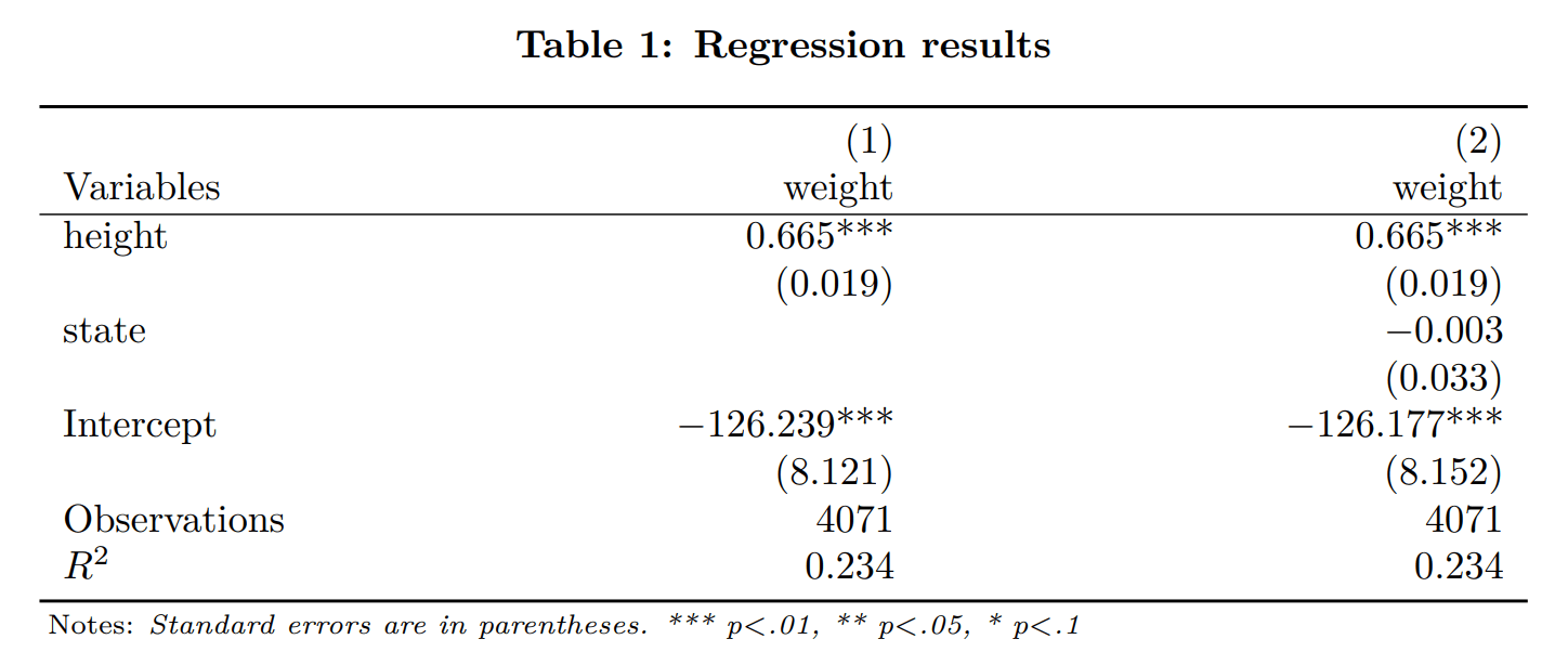
Start a new table with option reset
Option reset causes “asdocx” to make a new nested table, i.e., instead of appending to the existing nested table, option reset will start a new table in the existing file.
[code]* Load data from the web
webuse highschool
* First regression
asdocx regress weight height, nest replace
* Add a second regression to the same nested model
asdocx regress weight height state , nest
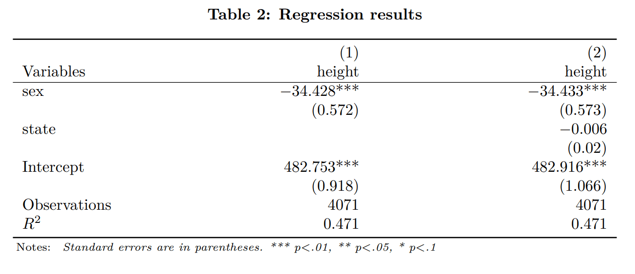
[/code]Next we are going to add the option reset to start a new nested table within the same document[code]
* Start a new nested model with option ‘reset’
asdocx regress height sex , nest reset
* Add a second regression the second nested model
asdocx regress height sex state , nest
[/code]